39 how to insert data labels in excel pie chart

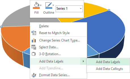
How to Make a Pie Chart in Excel - WinBuzzer Right-click your graph and choose "Add Data Labels" Your data will automatically appear on the pie segments Customize them by right clicking the graph and pressing "Format Data Labels…" Tick what... Customize data labels in pandas pie chart - Stack Overflow I am trying to create a python pie chart from a dataframe with customized data labels. The dataframe that I am working off of contains percentages the correspond to each of the pie chart sections. I would like to display those percentages as data labels rather than the percent values of the totals of the whole. Excel does allow me to do that.

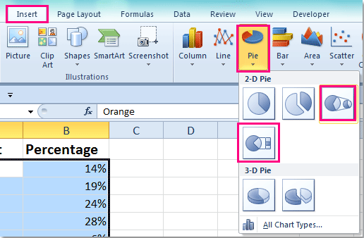
How To Create A Pie Chart In Excel - PieProNation.com With everything we need in place, its time to create a pie chart using the pivot table you just built. Select any cell in your pivot table . Navigate to the Insert tab. Hit the Insert Pie or Doughnut Chart button. Under 2-D Pie, click Pie. Once you do that, Excel will automatically plot a pie graph using your pivot table.

How to insert data labels in excel pie chart

How to ☝️Make a Pie Chart in Excel (Free Template) How to Add Labels to a Pie Chart To make our circle chart a bit more informative, add some data labels illustrating the numeric value of each slice by right-clicking on your pie chart and choosing " Add Data Labels. " Once there, Excel will automatically generate dynamic data labels based on your actual values. excelunlocked.com › pie-of-pie-chart-in-excelPie of Pie Chart in Excel - Inserting, Customizing - Excel ... Jan 03, 2022 · In the above example, there were a total of 6 data points. The Parent Pie chart represents three of them i.e Facebook, Youtube, and Instagram while the fourth data point named “Other” splits into a subset Pie chart that represents the rest of the three data points i.e Zee, Linkedin, and Hotstar. how to change legend name in excel pie chart To remove the labels, select the None command. By default the legend text is based on the column headings in the data on which. Select the data that you will use to create the pie

How to insert data labels in excel pie chart. How To Make A Pie Chart In Excel - PieProNation.com Enter the data in an excel sheet. Select the range of data ie., A1: B8 then click on Insert tab in the Ribbon and click on the Pie Chart icon in the Charts section and select the first chart under 2-D Pie Option. The Pie Chart looks like as given below: This is how the 2D pie chart looks like. Make Me A Pie Chart - PieProNation.com To rotate a pie chart in Excel, do the following: Right-click any slice of your pie graph and click Format Data Series. On the Format Data Point pane, under Series Options, drag the Angle of first slice slider away from zero to rotate the pie clockwise. Or, type the number you want directly in the box. › charts › axis-labelsHow to add Axis Labels (X & Y) in Excel & Google Sheets Excel offers several different charts and graphs to show your data. In this example, we are going to show a line graph that shows revenue for a company over a five-year period. In the below example, you can see how essential labels are because in this below graph, the user would have trouble understanding the amount of revenue over this period. Create Pie Chart In Excel - PieProNation.com Select the data you will create a pie chart based on, click Insert > I nsert Pie or Doughnut Chart > Pie. See screenshot: 2. Then a pie chart is created. Right click the pie chart and select Add Data Labels from the context menu. 3. Now the corresponding values are displayed in the pie slices.

› pie-chart-in-excelPie Chart in Excel | How to Create Pie Chart | Step-by-Step ... Step 1: Select the data to go to Insert, click on PIE, and select 3-D pie chart. Step 2: Now, it instantly creates the 3-D pie chart for you. Step 3: Right-click on the pie and select Add Data Labels . Display data point labels outside a pie chart in a paginated report ... Create a pie chart and display the data labels. Open the Properties pane. On the design surface, click on the pie itself to display the Category properties in the Properties pane. Expand the CustomAttributes node. A list of attributes for the pie chart is displayed. Set the PieLabelStyle property to Outside. Set the PieLineColor property to Black. spreadsheeto.com › pie-chartHow To Make A Pie Chart In Excel: In Just 2 Minutes [2022] How To Make A Pie Chart In Excel. In Just 2 Minutes! Written by co-founder Kasper Langmann, Microsoft Office Specialist. The pie chart is one of the most commonly used charts in Excel. Why? Because it’s so useful 🙂. Pie charts can show a lot of information in a small amount of space. They primarily show how different values add up to a whole. How to ☝️Create a Male/Female Pie Chart in Excel Step 6. Create Data Labels. Another helpful option that you can add to your pie chart is to include data labels. It will make it easier to read because people won't have to keep looking from the legend to the pie in order to match the colors. Here's the quickest way to do it: 25. Click your pie chart to select it.

Chart.ApplyDataLabels method (Excel) | Microsoft Docs For the Chart and Series objects, True if the series has leader lines. Pass a Boolean value to enable or disable the series name for the data label. Pass a Boolean value to enable or disable the category name for the data label. Pass a Boolean value to enable or disable the value for the data label. How to Create Bar of Pie Chart in Excel - Computing.NET Step 1: Highlight the entire range. Step 2: Click on the Insert tab, Step 3: Navigate to the Chart grouping and click on the Insert Pie or Doughnut Chart icon. A drop-down box of Pie options is displayed. Step 4: Select the Bar of a Pie icon under the 2D pie category. This creates the combination as shown below. How to Create Pie of Pie Chart in Excel? - GeeksforGeeks Creating Pie of Pie Chart in Excel: Follow the below steps to create a Pie of Pie chart: 1. In Excel, Click on the Insert tab. 2. Click on the drop-down menu of the pie chart from the list of the charts. 3. Now, select Pie of Pie from that list. Below is the Sales Data were taken as reference for creating Pie of Pie Chart: Show data in a line, pie, or bar chart in canvas apps - Power Apps Add a pie chart. On the Insert tab, select Charts, and then select Pie Chart. Move the pie chart under the Import data button. In the pie-chart control, select the middle of the pie chart: Set the Items property of the pie chart to this expression: ProductRevenue.Revenue2014. The pie chart shows the revenue data from 2014.

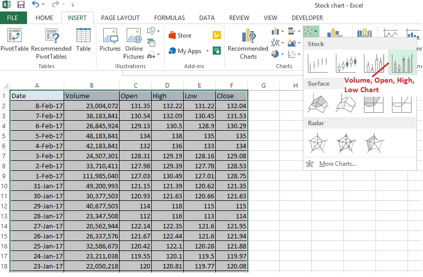
Stock chart in Excel or candlestick chart in Excel - DataScience Made Simple

How to Create a Pie Chart in Google Sheets (With Example) Step 3: Customize the Pie Chart. To customize the pie chart, click anywhere on the chart. Then click the three vertical dots in the top right corner of the chart. Then click Edit chart: In the Chart editor panel that appears on the right side of the screen, click the Customize tab to see a variety of options for customizing the chart.

Creating a 3D Pie Chart in Excel Vid.wmv - YouTube

Create A Pie Chart From Excel Data - PieProNation.com How To Create A Pie Chart. Just like any chart, we can easily create a pie chart in Excel version 2013, 2010 or lower. First, we select the data we want to graph. Click Insert tab, Pie button then choose from the selection of pie chart types: Pie, Exploded Pie, Pie of pie, Bar of pie, or 3D pie chart. Figure 2.

How to Insert Charts into an Excel Spreadsheet in Excel 2013

how to change legend name in excel pie chart judge dredd warzone skin. presentations . live events . websites . design . video

Everything You Need to Know About Pie Chart in Excel

› 2015/11/12 › make-pie-chart-excelHow to make a pie chart in Excel - Ablebits Nov 12, 2015 · Adding data labels to Excel pie charts. In this pie chart example, we are going to add labels to all data points. To do this, click the Chart Elements button in the upper-right corner of your pie graph, and select the Data Labels option. Additionally, you may want to change the Excel pie chart labels location by clicking the arrow next to Data ...

Excel 3-D Pie Charts - Microsoft Excel 2013

How To Make a Pie Chart in Excel (With Tips) | Indeed.com First, right-click on the pie chart and select "Add data labels" to insert the numerical value of each piece onto the pie chart. If you want your pieces to show category names, you can edit them by right-clicking any label and selecting "Format data labels," followed by "Label options."

4.1.3 Choosing a Chart Type: Pie Chart – Excel For Decision Making

how to group data in excel pie chart - perfectvisionksa.com See screenshot: 3. However, with an add-in like ChartExpo, it becomes extremely easy to visualize Likert data. How to Make a Pie Chart in Excel: 10 Steps (with Pictures) Source: display leader lines in pie chart, you just need to check an option then drag the labels out. chart in Excel

How to create pie of pie or bar of pie chart in Excel?

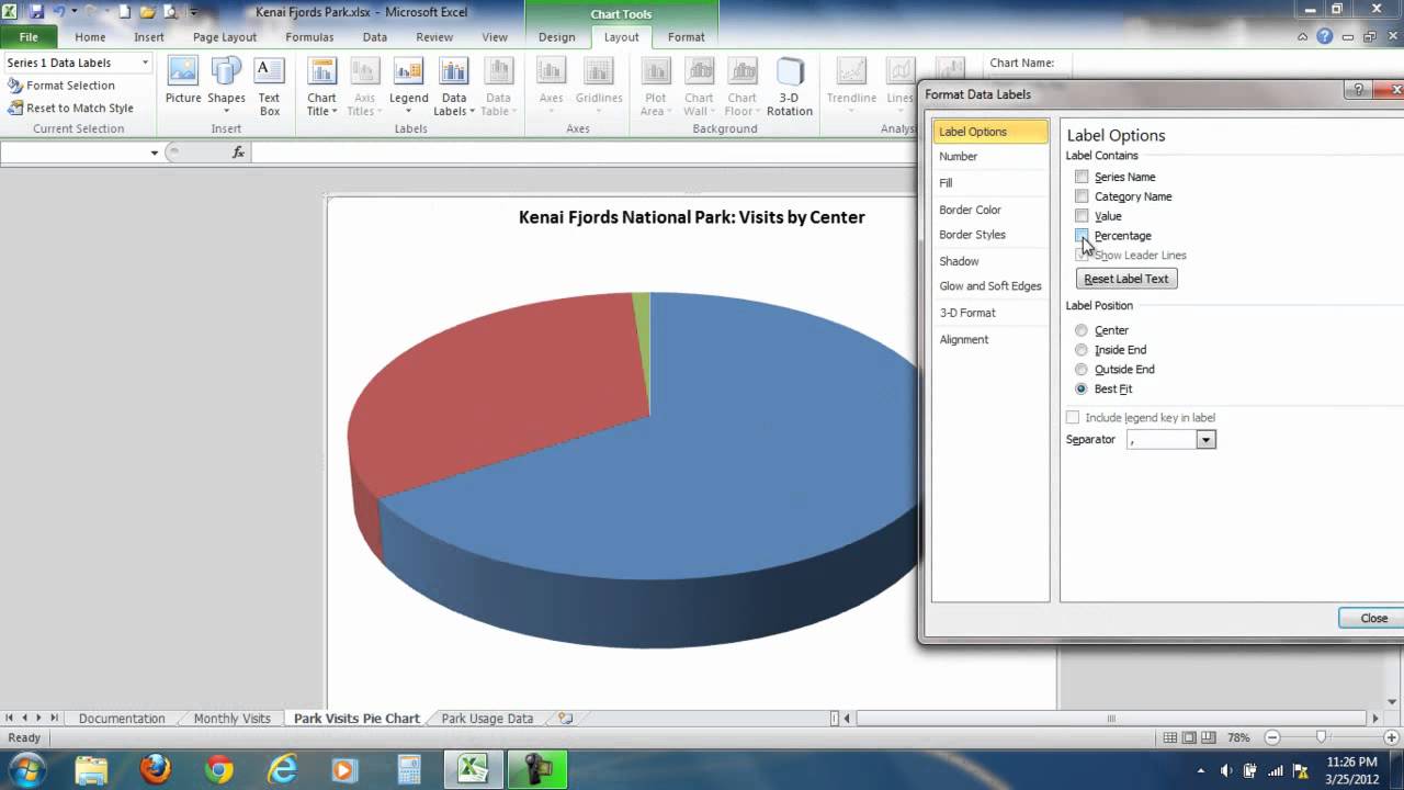
How to Show Percentage in Pie Chart in Excel? - GeeksforGeeks The steps are as follows : Select the pie chart. Right-click on it. A pop-down menu will appear. Click on the Format Data Labels option. The Format Data Labels dialog box will appear. In this dialog box check the "Percentage" button and uncheck the Value button. This will replace the data labels in pie chart from values to percentage.

Excel 3-D Pie Charts

excel - How to not display labels in pie chart that are 0% - Stack Overflow Generate a new column with the following formula: =IF (B2=0,"",A2) Then right click on the labels and choose "Format Data Labels". Check "Value From Cells", choosing the column with the formula and percentage of the Label Options. Under Label Options -> Number -> Category, choose "Custom". Under Format Code, enter the following:

Share :