42 how to create a scatter plot in excel with labels

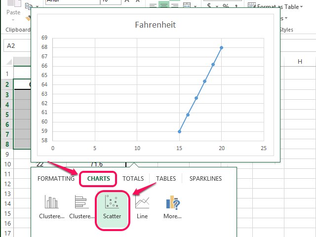
How to display text labels in the X-axis of scatter chart in Excel? Display text labels in X-axis of scatter chart. Actually, there is no way that can display text labels in the X-axis of scatter chart in Excel, but we can create a line chart and make it look like a scatter chart. 1. Select the data you use, and click Insert > Insert Line & Area Chart > Line with Markers to select a line chart. See screenshot: 2. Microsoft Excel - Creating a Scatter Plot with trend line and axis labels A video demonstrating how to create a scatter plot, with title axis labels, and trend line on Microsoft Excel. (Also a little extra at the end on printing)

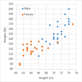
Creating Scatter Plot with Marker Labels - Microsoft Community Hi, Create your scatter chart using the 2 columns height and weight. Right click any data point and click 'Add data labels and Excel will pick one of the columns you used to create the chart. Right click one of these data labels and click 'Format data labels' and in the context menu that pops up select 'Value from cells' and select the column ...

How to create a scatter plot in excel with labels

toptipbio.com › forest-plot-microsoft-excelHow To Create A Forest Plot In Microsoft Excel - Top Tip Bio Note, that the study with the smallest Position value will be placed at the bottom of the forest plot. 3. Add a scatter plot to your graph. The next step is to use these new Position values to create a scatter plot, so it looks more like a forest plot. So, right-click on the graph and go to Select Data. Then you want to add a new Series. How to Make a Scatter Plot in Excel (Step-By-Step) | Create Scatter ... To create or make Scatter Plots in Excel you have to follow below step by step process, Select all the cells that contain data. Click on the Insert tab. Look for Charts group. Under Chart group, you will find Scatter (X, Y) Chart. Click the arrow to see the different types of scattering and bubble charts. You can pause the pointer on the icons ... How to use a macro to add labels to data points in an xy scatter chart ... Press ALT+Q to return to Excel. Switch to the chart sheet. In Excel 2003 and in earlier versions of Excel, point to Macro on the Tools menu, and then click Macros. Click AttachLabelsToPoints, and then click Run to run the macro. In Excel 2007, click the Developer tab, click Macro in the Code group, select AttachLabelsToPoints, and then click ...

How to create a scatter plot in excel with labels. › add-vertical-line-excel-chartAdd vertical line to Excel chart: scatter plot, bar and line ... May 15, 2019 · Select your source data and create a scatter plot in the usual way (Inset tab > Chats group > Scatter). Enter the data for the vertical line in separate cells. In this example, we are going to add a vertical average line to Excel chart, so we use the AVERAGE function to find the average of x and y values like shown in the screenshot: How to create a scatter plot and customize data labels in Excel During Consulting Projects you will want to use a scatter plot to show potential options. Customizing data labels is not easy so today I will show you how th... How to Make a Scatter Plot in Excel and Present Your Data Add Labels to Scatter Plot Excel Data Points. You can label the data points in the X and Y chart in Microsoft Excel by following these steps : Click on any blank space of the chart and then select the Chart Elements (looks like a plus icon). Then select the Data Labels and click on the black arrow to open More Options. Labeling X-Y Scatter Plots (Microsoft Excel) Just enter "Age" (including the quotation marks) for the Custom format for the cell. Then format the chart to display the label for X or Y value. When you do this, the X-axis values of the chart will probably all changed to whatever the format name is (i.e., Age). However, after formatting the X-axis to Number (with no digits after the decimal ...

How to Make a Scatter Plot in Excel? 4 Easy Steps Option 1: Plot both variables in X vs Y scatter plot style. Use this option to check for linear relationships between variables. To implement this, just select the range of the two variables. Option 1: Select the two continuous variables. Option 2 involves plotting the variables separately in two different series. A step-by-step guide to creating a scatter plot in Excel - AilCFH 2. Display the scatter map. After entering the data, select the columns you want, go to the Insert tab in Excel, select the XY Scatter Chart, and choose the first Scatter Chart option. Now you should have a scatter chart in your Excel file. Once you've done this, you'll need to add a chart title to the scatter plot. Add Custom Labels to x-y Scatter plot in Excel Step 1: Select the Data, INSERT -> Recommended Charts -> Scatter chart (3 rd chart will be scatter chart) Let the plotted scatter chart be. Step 2: Click the + symbol and add data labels by clicking it as shown below. Step 3: Now we need to add the flavor names to the label. Now right click on the label and click format data labels. Use text as horizontal labels in Excel scatter plot Edit each data label individually, type a = character and click the cell that has the corresponding text. This process can be automated with the free XY Chart Labeler add-in. Excel 2013 and newer has the option to include "Value from cells" in the data label dialog. Format the data labels to your preferences and hide the original x axis labels.

How to Create a Scatter Plot in Excel - dummies To create a scatter chart of this information, take the following steps: Select the worksheet range A1:B11. On the Insert tab, click the XY (Scatter) chart command button. Select the Chart subtype that doesn't include any lines. Excel displays your data in an XY (scatter) chart. Confirm the chart data organization. How to add labels to the mosaic plot - Microsoft Excel 2016 This is the third, and last part of the tip How to create a mosaic plot in Excel (the second part is How to create a step Area chart for the mosaic plot). The step area chart created in the previous part has invalid labels for both axes and no data labels: ... There are at least two types of labels that are parts of the mosaic plot: Data labels ... How to Add Labels to Scatterplot Points in Excel - Statology Step 3: Add Labels to Points. Next, click anywhere on the chart until a green plus (+) sign appears in the top right corner. Then click Data Labels, then click More Options…. In the Format Data Labels window that appears on the right of the screen, uncheck the box next to Y Value and check the box next to Value From Cells. › q-q-plot-excelHow to Create a Q-Q Plot in Excel - Statology Mar 27, 2020 · Example: Q-Q Plot in Excel. Perform the follow steps to create a Q-Q plot for a set of data. Step 1: Enter and sort the data. Enter the following data into one column: Note that this data is already sorted from smallest to largest. If your data is not already sorted, go to the Data tab along the top ribbon in Excel, then go to the Sort & Filter ...

Make Technical Dot Plots in Excel | LaptrinhX

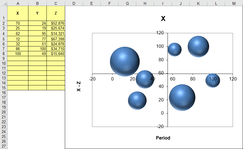
How to Make a Scatter Plot in Excel with Multiple Data Sets? So, for the first data set, they tested the cash-out charge. To make a scatter plot, select the data set, go to Recommended Charts from the Insert ribbon and select a Scatter (XY) Plot. Press ok and you will create a scatter plot in excel. In the chart title, you can type fintech survey.

Scatter Plot Template in Excel | Scatter Plot Worksheet

How to Create Scatter Plots in Excel (In Easy Steps) To create a scatter plot with straight lines, execute the following steps. 1. Select the range A1:D22. 2. On the Insert tab, in the Charts group, click the Scatter symbol. 3. Click Scatter with Straight Lines. Note: also see the subtype Scatter with Smooth Lines. Note: we added a horizontal and vertical axis title.

How to Create a Scatter Plot in Excel

How to Make a Scatter Plot in Excel with Two Sets of Data? To get started with the Scatter Plot in Excel, follow the steps below: Open your Excel desktop application. Open the worksheet and click the Insert button to access the My Apps option. Click the My Apps button and click the See All button to view ChartExpo, among other add-ins.

How to Make an XY Graph on Excel | Techwalla.com

How to Create a Scatterplot with Multiple Series in Excel Step 3: Create the Scatterplot. Next, highlight every value in column B. Then, hold Ctrl and highlight every cell in the range E1:H17. Along the top ribbon, click the Insert tab and then click Insert Scatter (X, Y) within the Charts group to produce the following scatterplot: The (X, Y) coordinates for each group are shown, with each group ...

Fors: Adding labels to Excel scatter charts

How to Combine Two Scatter Plots in Excel (Step by Step Analysis) 7 Easy Steps to Combine Two Scatter Plots in Excel. Step 1: Use the Charts Ribbon to Select Scatter Option. Step 2: Select Data to Create the First Scatter Plot. Step 3: Add Another Series to Combine Two Scatter Plots. Step 4: Change the Layout of Two Combined Scatter Plots. Step 5: Add Secondary Horizontal/Vertical Axis to Combined Scatter Plots.

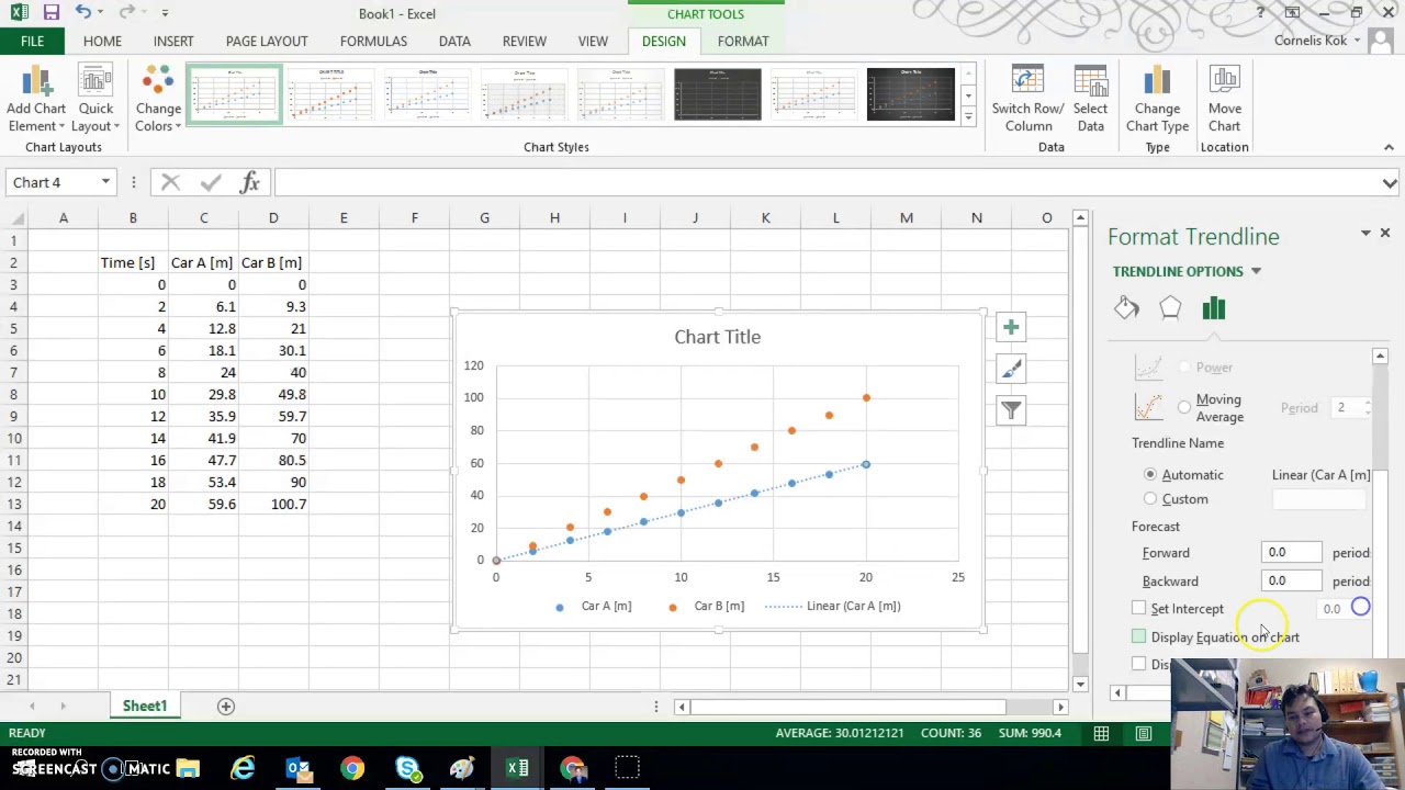
Microsoft Excel - Creating a Scatter Plot with trend line and axis ...

Scatter Plots in Excel with Data Labels Select "Chart Design" from the ribbon then "Add Chart Element" Then "Data Labels". We then need to Select again and choose "More Data Label Options" i.e. the last option in the menu. This will ...

How to Create a Scatter Plot in Excel - TurboFuture - Technology

Improve your X Y Scatter Chart with custom data labels Go to tab "Insert". Press with left mouse button on the "scatter" button. Press with right mouse button on on a chart dot and press with left mouse button on on "Add Data Labels". Press with right mouse button on on any dot again and press with left mouse button on "Format Data Labels". A new window appears to the right, deselect X and Y Value.

How to join the points on a scatter plot in Excel - YouTube

How to label scatterplot points by name? - Stack Overflow Apr 13, 2016 — right click on your data point · select "Format Data Labels" (note you may have to add data labels first) · put a check mark in "Values from Cells ...5 answers · Top answer: Well I did not think this was possible until I went and checked. In some previous version of ...How to label scatter point plots from data column in excelJul 23, 2017Use text as horizontal labels in Excel scatter plot - Stack ...Jun 11, 2017How to create a scatter plot in excel based on time? - Stack ...Apr 1, 2022Change horizontal axis labels in XY Scatter chart with VBASep 21, 2020More results from stackoverflow.com

Share :